Lab 3: Numerical Methods: Roots and Fractals
This labs explores algorithmic techniques for successive approximations to the square root function. This includes the bisection method and Newton's method. Moving beyond square roots to the complex cube roots of unity, this lab also explores ways of visualizing common areas of convergence resulting in a well-known Julia set called the Newton basin.
Step 1: Source Code
- This week we will use a python package
called matplotlib, which is installed in the
system. The first time it is imported, it builds a
local font cache. This process can take a few minutes. Let's
get it started. Start python3 and type
>>> import matplotlib.pyplot as plt
While this is loading you can open another terminal window and continue with the process. - Clone your private repo to an appropriate directory in your home folder
(
~/labsis a good choice):$ git clone git@github.com:williams-cs/<git-username>-cs135-lab3.git
Remember, you can always get the repo address by using the ssh copy-to-clipboard link on github. - Once inside your <git-username>-cs135-lab3 directory, create a virtual environment using
$ virtualenv --system-site-packages -p python3 venv
The --system-site-packages will let us use the matplotlib package. - Activate your environment by typing:
$ . venv/bin/activate
- Use pip to install the pillows imaging library:
$ pip install pillow
- Remember that you must always activate your virtual environment when opening a new terminal
Step 2: Calculating Square Roots using Successive Approximations
The file sqrt.py contains function headers
for sqrt_newton and sqrt_bisect.
Implement these functions using x/2 as the starting
value in sqrt_newton and the values 0
and x as the starting low and high values
respectively in sqrt_bisect.
    def sqrt_newton(x, iter):
        """
        Use Newton's Method for 'iter' iterations
        to approximate sqrt(x)
        """
    def sqrt_bisect(x, iter):
        """
        Use bisection / binary search method for 'iter' iterations
        to approximate sqrt(x)
        """
You can always test your functions out by
running python in interpreter mode and typing
	>>> import sqrt
	>>> sqrt.sqrt_newton(25,3)
	5.011394106532552
	>>> sqrt.sqrt_bisect(25,3)
	4.6875
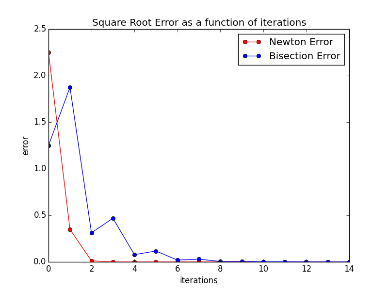
Implement the functions absolute_error, list_of_errors, and
save_plot. You will find the matplotlib
function plt.savefig("somefile.png") useful for saving the current plot to
disk. Below you will also find a picture of the plot that you can use as a guide when
coding the save_plot function.
    def absolute_error(square, iterations, sqrt_fn):
      """
      Calculate the absolute error between the value reported by
      'sqrt_fn' and the actual square root of 'square'.  Absolute error is the absolute
      difference between the correct square root and the value given by 'sqrt_fn' after
      'iterations'"""
    def list_of_errors(square, max_iterations, sqrt_fn):
      """
      Return a list of 'max_iterations' absolute error values for 'sqrt_fn' where
      the error value at index i represents the absolute error between 'sqrt_fn'
      on 'square' after i iterations and the actual square root.
      """
    def save_plot(newton_err, bisect_err, filename):
      """
      Save a figure to 'filename' that shows absolute error with respect to
      number of iterations for both Newton's method and the bisection method.
      """
Calling
$ python sqrt.py 25 15 error.png
from the command line
should produce a file called error.png that you can open
in Preview by typing $ open error.png. It should
look like this:
Step 3: Making Images
Included in this week's source code is a module called image.py that provides a simple interface for creating images, drawing points, and saving images.
    from PIL import Image, ImageDraw

    def create_image(width, height):
      return Image.new("RGB", (width, height), (255, 255, 255))

    def draw_point(image, x, y, color):
      ImageDraw.Draw(image).point((x,y), color)

    def save_image(image, filename):
      image.save(filename, "PNG")
We can use the above interface to create images. For example, here's a 100x100 pixel image with a 20-pixel wide horizontal stripe. Note that the coordinate system for images runs from top-left (0,0) to bottom-right (100,100). Colors are just 3-tuples of RGB (Red, Green, and Blue) values that each range from 0 to 255.
      >>> im = image.create_image(100,100)
      >>> for x in range(100):
      ...   for y in range(40,60):
      ...     image.draw_point(im, x, y, (255, 0, 0))
      ...
      >>> image.save_image(im, "redstripe.png")

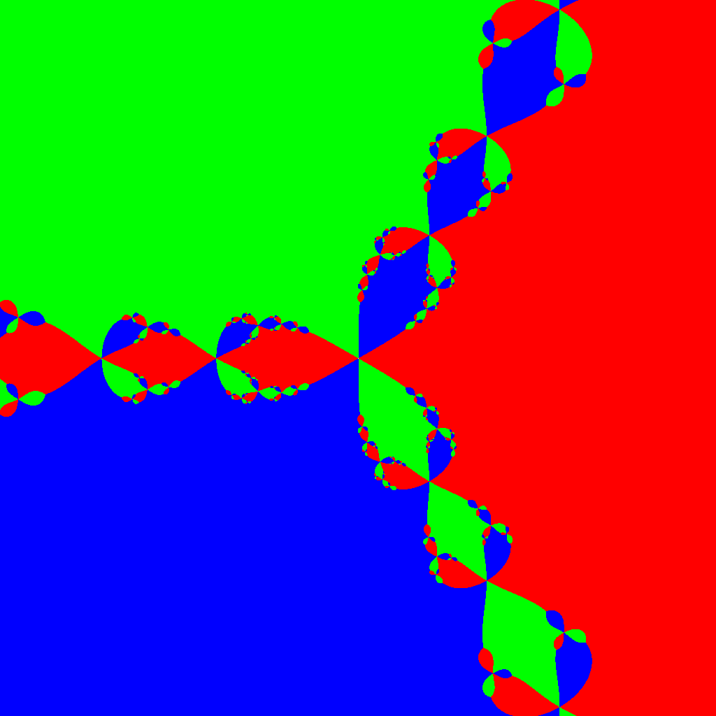
Step 4: Newton's Basin
If z is a complex number then the function f(z)=z3-1 has three different complex roots at
- (1,0)
- (-1/2, √3/2)
- (-1/2, -√3/2)
To which root Newton's method converges depends entirely on the point at which it starts. Surprisingly, this starting point is very sensitive. In fact, if one visualizes the complex plane so that one colors each complex point according to the root on which it converges using Newton's method, you obtain the following fractal known as Newton's fractal
Recall that for some polynomial f(z), Newton's method finds successive approximations of a root of f(z) by letting the approximation zn at iteration n be given by the following assignment:
zn = zn-1 - f(zn-1) / f'(zn-1)
so for f(z)=z3-1 this translates to
zn = zn-1 - (zn-13-1) / 3(zn-12)
Examine the source code in basin.py. One function closest_root, is defined for you. Three others you must define.
You should interpret the interpolate_value functions as taking a value x in the range [0,length-1] and returning the corresponding position in the range (y1,y2). That is you should return y1 + (x / length * (y2 - y1))
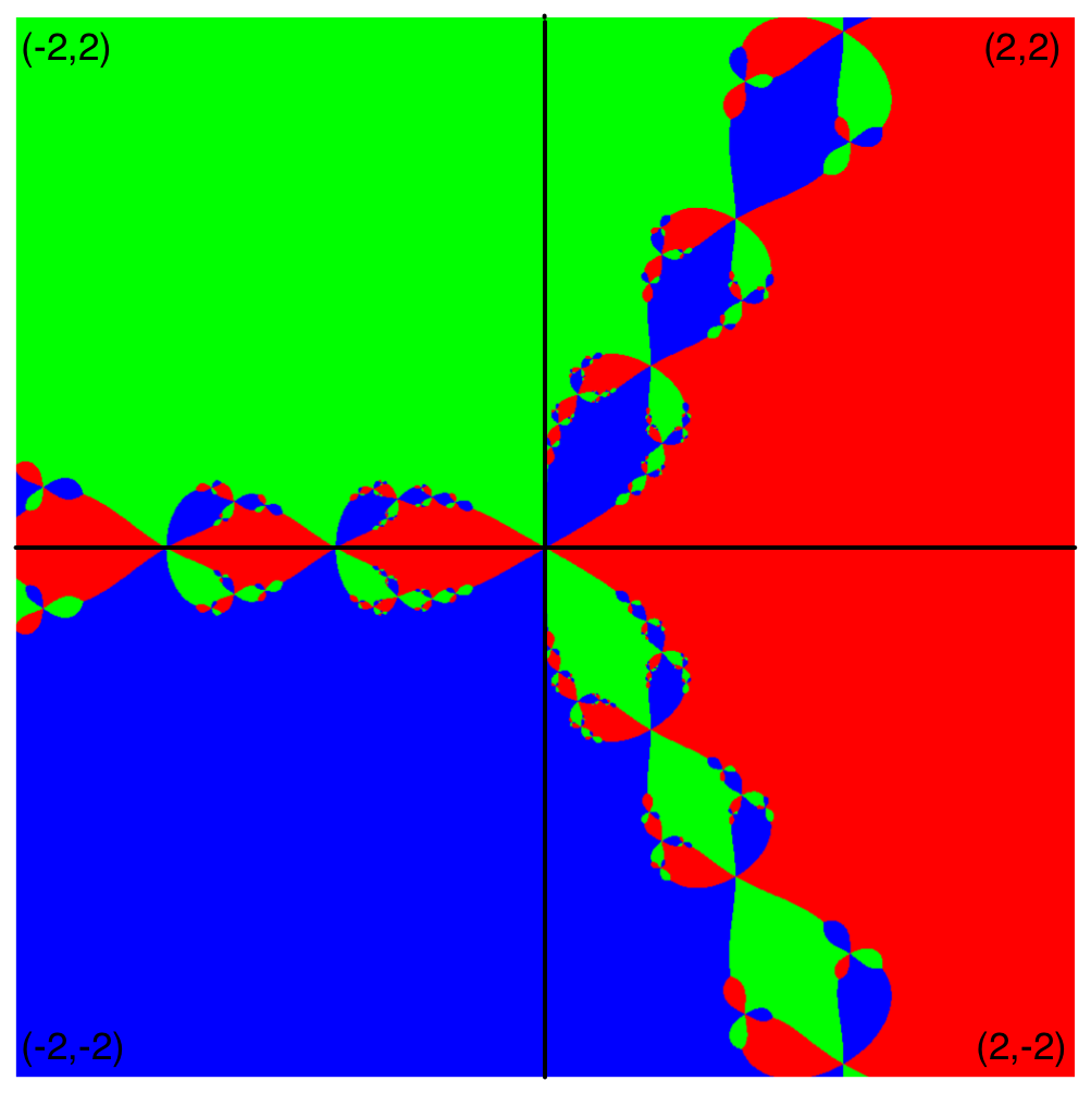
In particular, the draw function should do the following:
- Create an image with dimesions IMAGE_WIDTH x IMAGE_HEIGHT uing the image module
- For each pixel (i,j) in the image, linearly interpolate that pixel into the complex plane. To do this, you should make two calls to interpolate_value. The top-left corner of the image should correspond to the bttom-left corner of the complex plane.
- If the pixel gets interpolated to (0,0) then skip it.
- Given the complex point, check to
which root it converges using Newton's method. Color the
pixel
- RED if it's ZROOT1,
- BLUE if it's ZROOT2, and
- GREEN if it's ZROOT3.
- Save the resuling image as filename
    def cube_root_of_unity(z, iter):
        """Use Newtown's Method for 'iter' iterations
           to find a cube root of unity.  Start the approximation
           at point z"""
    def interpolate_value(x,length,y1,y2):
        """Linearly interpolate the value x in the range [0,length-1]
           to range [y1,y2]"""
    def draw(output):
        """
        1.  Create an image with dimesions IMAGE_WIDTH x IMAGE_HEIGHT
        2.  For each pixel (i,j) in the image, linearly interpolate
            that pixel into the complex plane.  The top-left corner
            of the image should correspond to the bttom-left corner
            of the complex plane.
        3.  If the pixel gets interpolated to (0,0) then skip it.
        4.  Given the complex point, check to which root it converges
            using Newton's method.  Color the pixel
            (a) RED if it's ZROOT1,
            (b) BLUE if it's ZROOT2, and
            (c) GREEN if it's ZROOT3
        5.  Save the resuling image as 'filename'"""
You should be able to run
$ python basin.py basin.pngand produce the image below.