What’s In A Name?

Objectives

In this lab we will look at data from the Social Security Administration ¹ about the popularity of baby names from 1880-2021. In doing so, you will gain experience with the following:

• Using dictionaries in Python
• Plotting data using Python’s matplotlib library
• Reading data from CSV (comma separated values) files

Getting Started

Before you begin, clone this week’s repository in the usual manner:

git clone https://evolene.cs.williams.edu/cs134-labs/23xyz3/lab06.git ~/cs134/lab06

where your CS username replaces 23xyz3.

If you are using a personal computer, for this lab you will need to have installed matplotlib. This was part of the personal machine setup instructions. The lab machines are already configured for you.

Processing the Data

The Social Security Administration collects data on the frequency of first names assigned at birth in the U.S. In the data/namesDataAll.csv data file, you will find comma-delimited records containing this data. Some notes on the format of this data:

• Each line has the format “year,name,sex,number”, where
  • year is 1880 to 2021
  • name is 2 to 15 characters
  • sex is M (male) or F (female), and
  • number is the number of occurrences of the name.
• The data is sorted numerically by year.
• The data only includes names with at least 5 occurrences.
• All names start with a capital letter.

For reference, here are the first few lines of the file:

1880,Mary,F,7065
1880,Anna,F,2604
1880,Emma,F,2003
1880,Elizabeth,F,1939
1880,Minnie,F,1746
1880,Margaret,F,1578

To effectively process the data from this file, we will utilize two helper functions: trim() and split().

The function trim takes one argument: line (a string). If line ends with a newline character, then trim returns a new string that is identical to line, but without the final newline character. Otherwise, it just returns line.

    >>> trim("Hello there!\n")
    'Hello there!'
    >>> trim("Hello there!!")
    'Hello there!!'
    >>> trim("")
    ''

The function split takes one argument: comma_separated_string. The comma_separated_string is a specially formatted string and consists of substrings separated by a comma (and does not end in a comma). It returns a list of its component substrings.

Here are some examples of its usage:

    >>> split('a,b,c,d')
    ['a', 'b', 'c', 'd']
    >>> split('alpha,bravo,charlie')
    ['alpha', 'bravo', 'charlie']
    >>> split('alpha')
    ['alpha']
    >>> split("")
    []

Note: We have provided implementations of the above functions in file_utils.py. These are re-implementations of existing string methods in Python (called strip and split). We will be discussing methods and how to use them in lectures soon. But for this lab, you should use these helper functions by importing them into the files that you are writing your code using a properly formatted import statement (discussed below) and then calling the imported functions.

Organizing the Data

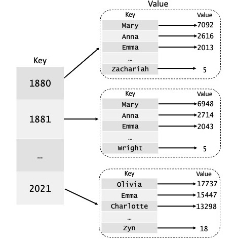
At the start of runtests.py, you will find two useful examples of the ways we will organize the above data in this lab: name tables and year tables.

Name Tables

A name table tells us how many times a newborn baby was given a particular first name in a particular year. A name table is implemented as a dict whose keys are strs (the baby names) and whose values are ints (the number of babies that were given that name). In runtests.py, the function example_name_table1 returns the following example of a name table:

{'William': 1000, 'Lida': 19, 'Shikha': 3}

This means that in a particular year, 1000 babies were named William, 19 babies were named Lida, and 3 babies were named Shikha.

Year Tables

A year table associates each year with its respective name table:

A year table is implemented as a dict whose keys are ints (the years) and whose values are dicts (the name table associated with each year). In runtests.py, the function example_year_table1 returns the following example of a year table:

{1974: {'William': 4000, 'Lida': 20, 'Shikha': 3},
 1975: {'William': 3000, 'Lida': 14, 'Shikha': 2},
 1976: {'William': 2000, 'Lida': 10, 'Shikha': 5},
 1977: {'William': 1000, 'Lida': 19, 'Shikha': 7},
 1978: {'William': 500, 'Lida': 13, 'Shikha': 4},
 1979: {'William': 200, 'Lida': 16, 'Shikha': 1}}

This means that:

• in 1974, 4000 babies were named William, 20 babies were named Lida, and 3 babies were named Shikha
• in 1975, 3000 babies were named William, 14 babies were named Lida, and 2 babies were named Shikha
• etc.

What You Need To Do For This Lab

Q1: Read real-world data

Review the documentation and implementation of trim and split and then import these functions by including the following import command at the top of names.py:

from file_utils import trim, split

Using these helper functions, complete the implementation of the function read_names in names.py. When given a filename (e.g. data/namesDataAll.csv), this function should read the contents of that CSV file. It should also create and return a year table (a dict of dicts, see the previous section “Organizing the Data” for specifics) containing the data found in the file. When you read in the data, make sure you convert both the years and frequencies to integers. If multiple entries exist for a name in a given year (such as an entry for the same name as both M and F), the totals for the name should be summed in the dictionary.

You can test your implementation in interactive Python:

>>> from names import *
>>> year_table = read_names("data/namesDataAll.csv")
>>> year_table[2021]["Emily"]
6547
>>> year_table[1880]["Emily"]
210
>>> 1900 in year_table
True
>>> 1600 in year_table
False
>>> len(year_table[1880])
1889

Alternatively, you can type the following into the Terminal:

python3 runtests.py q1

Q2: Compute the popularity of a name over time

Implement the name_frequency function in names.py, which takes three arguments:

• a year table (see the above section “Organizing the Data” for the definition of a year table) called year_table
• a str called name
• a list of ints called years

It should return a list of ints corresponding to the frequency of the provided name across the specified years. If a year does not exist in the year table or a name does not exist in the name table associated with a particular year, you should use the value 0 for that year in your list.

You can test your implementation in interactive Python:

>>> from runtests import *
>>> from names import *
>>> name_frequency(example_year_table1(), "William", [1977, 1978, 1979])
[1000, 500, 200]
>>> name_frequency(example_year_table1(), "Lida", [1977, 1979])
[19, 16]

Alternatively, you can type the following into the Terminal:

python3 runtests.py q2

To further demonstrate that your implementation of name_frequency is correct, modify the function example_year_table2 in runtests.py so that it creates and returns a year table that might catch errors that example_year_table1 does not catch. Then, add at least one new test of your own design to runtests.py that uses your new example year table (we have provided an incomplete def statement called my_name_frequency_test in the YOUR EXTRA TESTS section for you to complete).

When creating your new example year table and associated test(s), think about what cases the original table isn’t capturing. For instance, the names “William”, “Lida”, and “Shikha” appear in every name table, but this doesn’t have to be the case. Would your code for name_frequency still work correctly if the name “Lida” didn’t appear in the 1978 name table or if the year 1234 did not exist in the data?

Q3: Compute the popularity of first initials in a given year

Implement the function letter_frequency, which takes two arguments:

• a year table (see the above section “Organizing the Data” for the definition of a year table) called year_table
• a int called year. You may assume that year is a key in year_table.

It should return a list of integer frequencies indicating how many babies received a name starting with each letter. Remember to take the frequency of the name into account, as well; that is, if “Mary” shows up 50 times, the letter “M” should be incremented by 50 when processing “Mary”.

The resulting list returned by your function should have 26 entries corresponding to the frequency of each letter in the alphabet in alphabetical order. For example, in your resulting list, entry 0 should correspond to the frequency of names that start with “A”, index 1 should correspond to the frequency of names that start with “B”, and so on. You may assume that every name starts with a capital letter. If no names started with a particular letter, then the list element corresponding to that letter should be 0.

You can test your implementation in interactive Python:

>>> from runtests import *
>>> from names import *
>>> letter_frequency(example_year_table1(), 1978)
[0, 0, 0, 0, 0, 0, 0, 0, 0, 0, 0, 13, 0, 0, 0, 0, 0, 0, 4, 0, 0, 0, 500, 0, 0, 0]
>>> letter_frequency(example_year_table1(), 1979)
[0, 0, 0, 0, 0, 0, 0, 0, 0, 0, 0, 16, 0, 0, 0, 0, 0, 0, 1, 0, 0, 0, 200, 0, 0, 0]

Alternatively, you can type the following into the Terminal:

python3 runtests.py q3

To further demonstrate that your implementation of letter_frequency is correct, please add at least one new test to runtests.py (we have provided an incomplete def statement called my_letter_frequency_test in the YOUR EXTRA TESTS section). Your test(s) should use the year table that you created in example_year_table2().

Again, when creating your test(s), think about what cases the original table isn’t capturing. For instance, the names “William”, “Lida”, and “Shikha” all begin with different letters. Does your code still work when provided with a year table that contains several names that start with the same letter?

Q4: Visualize baby name popularity over time

Implement the function plot_name_frequency in names.py.

This function takes three arguments:

• year_table: a year table (see the previous section “Organizing the Data” for the definition of a year table)
• name: a str specifying a particular baby name
• years: a list of ints, specifying the years that we want to plot

This function need not return anything. However, it should pop up a window that plots the year (x-axis) vs. the frequency of the specified baby name in that year (y-axis) using a line plot.

We have provided a partial implementation of plot_name_frequency, however it requires you to write additional code so that the variables x_values and y_values are initialized and assigned the appropriate values.

When implemented correctly, the plot showing the frequency of the name “Lida” over the time period covered by example_year_table1 will look like the following:

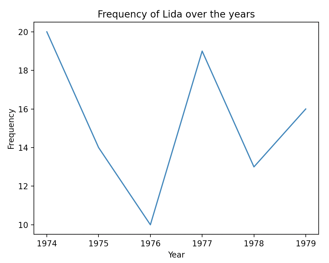
You can verify that your code produces the same figure by typing the following into interactive Python:

>>> from runtests import *
>>> from names import *
>>> plot_name_frequency(example_year_table1(), "Lida", [1974, 1975, 1976, 1977, 1978, 1979])

Alternatively, you can type the following into the Terminal:

python3 runtests.py q4

Q5: Visualize the popularity of first initials in a given year.

Implement the function plot_letter_frequency in names.py.

The plot_letter_frequency function takes two arguments:

• year_table: a year table (see the previous section “Organizing the Data” for the definition of a year table)
• year: an int that specifies the year that we are interested in analyzing

This function need not return anything. However, it should pop up a window that plots first initials (x-axis) vs.  the frequency of that initial in the specified year (y-axis) using a bar plot.

We have provided a partial implementation of plot_letter_frequency, however it requires you to write additional code so that the variables x_values and y_values are initialized and assigned the appropriate values.

When implemented correctly, this should be the plot comparing the frequency of initial letters in the year 1978, according to the data provided by example_year_table1:

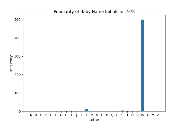
You can verify that your code produces the same figure by either typing the following into interactive Python:

>>> from runtests import *
>>> from names import *
>>> plot_letter_frequency(example_year_table1(), 1978)

Alternatively, you can type the following into the Terminal:

python3 runtests.py q5

Q6: Explore naming trends

Once your code is working, you can use it to visualize trends in how Americans have named their babies for the past century and a half. For instance, we can plot the popularity of the name Emma from 1880-2021 in interactive Python:

>>> from names import *
>>> year_table = read_names("data/namesDataAll.csv")
>>> years = list(range(1880, 2022))
>>> plot_name_frequency(year_table, name, years)

You should see the following graph:

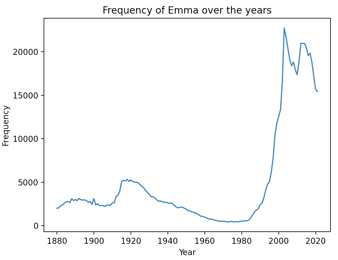
Note the surge in popularity around the year 2002, which is when Rachel named her baby “Emma” on the sitcom Friends.

Alternatively, you can generate this plot by typing the following into the Terminal:

python3 runtests.py q6 Emma

If you replace “Emma” with any other name, it will use your code to plot the popularity of that name over the same time period. Make sure that you start the name with a capital letter!

Q7: Animate your bar graph

As a final step, let’e explore how the frequency of first initials has changed over time. One interesting way to investigate this trend is by using an animated graph that cycles through the years in our data set. The code is provided for you to handle the animation. All you need to do is run python3 animation.py. However, this won’t work until your implementations in names.py are correct!

Your final output should look like this (but with the plot updating for each year over time):

Because the graphs show the absolute number of babies with a particular initial, you can also get a sense for the periods in American history when birth rates spiked. For instance, note that the bars grow substantially during the post-WWII Baby Boom from 1946 to 1964.

Submitting your work

When you’re finished, commit and push your work (names.py and runtests.py) to the server as in previous labs. (We will check to see that your script generates the desired plots; you do not need to submit the .png files.)

Note: There is nothing to submit for Q6 or Q7.

Functionality and programming style are important, just as both the content and the writing style are important when writing an essay. Make sure your variables are named well, and your use of comments, white space, and line breaks promote readability. We expect to see code that makes your logic as clear and easy to follow as possible.

Do not forget to add, commit, and push your work as it progresses! Test your code often to simplify debugging.